- Nidhi Kamra
Ages: 16 +
(P.S. if you would like a Word version of this, message me via the contact form or Twitter and I will send you the file.It's easier to read on Word as it has the proper formatting.)
Ages: 16 +
(P.S. if you would like a Word version of this, message me via the contact form or Twitter and I will send you the file.It's easier to read on Word as it has the proper formatting.)
I recently came across the K-word.
At first, my brain, being my brain, somersaulted at the thought of a freshly brewed cup of filtered coffee – steamed, extra hot, almond milk, stevia…
The pleasure didn’t last long. Words like covariance, Gaussian, probability, transpose, discrete linear filtering etc. spewed out at me, along with some very disturbing alien-like equations. Yuck.
I wanted to cry.
Really bad.
However, after reading on the topic from a few different sources, I decided to re-write and integrate them to make it easier for me to understand the big picture, in case I ever had to deal with it in a future life. Hopefully it will help someone else as well.
All references are mentioned at the end of the post.
We’ll start with the big picture and equations. Don’t let it daunt you. We’ll peel the onion layers to make sense of everything as far as possible. Remember, this is a very general overview.
Let’s dive in!
What the Hell Is It?
Proposed by R.E. Kalman in 1960, the Kalman Filter is a set of recursive equations that help predict (estimate) the next state of a system (Where will the robot move next?). The filter also incorporates and processes various measurement and prediction errors (called noise), and outputs the best possible estimate of the next state. The goal is to minimize the difference in error between the estimated values and the actual measured value of noisy sensor(s). Recursion is used in computer code and just means the output of an equation or function is fed back again into the same function.
The Kalman filter has a plethora of applications ranging from navigation (GPS), tracking objects (missiles, aircraft/ spacecraft, cars, faces…), economics, signal processing etc. It was also incorporated in NASA’s Apollo navigation system.
Various systems rely on different sensors or systems to provide them with input data. For example, an aircraft is detected by radar that can render erroneous / noisy data. GPS systems are prone to errors as the satellite signal travels from space into the atmosphere, and likely bounces off the ground to get to the GPS receiver. This also results in a noisy signal.
A drone may rely on inputs from the GPS, air data sensors, magnetic compasses etc. Each sensor has a limitation with respect to the type of data it provides and the noise/ error. To get an accurate estimate, it would be good to somehow combine the inputs of all these sensors and eliminate errors. Relying on the input from just one sensor and not knowing the exact location of where you are or going can cause trouble, and even more if a car / drone is autonomous!
Think about a medical condition and the plethora of treatment options available. To get the best treatment, you may consider consulting an MD, a naturopath, an energy healer, a homeopathic doctor etc. in order to ensure successful treatment. Each provider has his / her own specialization and provides a different perspective to optimize your health. That’s where the Kalman Filter comes in. It has a way of providing a best estimate of a state based on noisy sensors as well as their combined asynchronous inputs!
En route to the Prediction Equations – Keep Breathing Through It!
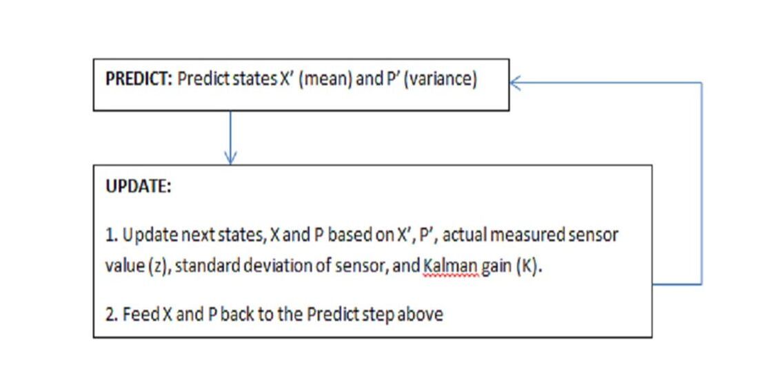
Let’s first define the flow state. The Kalman Filter has two easy steps: Predict and Update (predict the next state, update/correct the state from prediction by taking into account sensors and noise etc., and then use the updated state values to predict the next state (recursion)).
I recently came across the K-word.
At first, my brain, being my brain, somersaulted at the thought of a freshly brewed cup of filtered coffee – steamed, extra hot, almond milk, stevia…
The pleasure didn’t last long. Words like covariance, Gaussian, probability, transpose, discrete linear filtering etc. spewed out at me, along with some very disturbing alien-like equations. Yuck.
I wanted to cry.
Really bad.
However, after reading on the topic from a few different sources, I decided to re-write and integrate them to make it easier for me to understand the big picture, in case I ever had to deal with it in a future life. Hopefully it will help someone else as well.
All references are mentioned at the end of the post.
We’ll start with the big picture and equations. Don’t let it daunt you. We’ll peel the onion layers to make sense of everything as far as possible. Remember, this is a very general overview.
Let’s dive in!
What the Hell Is It?
Proposed by R.E. Kalman in 1960, the Kalman Filter is a set of recursive equations that help predict (estimate) the next state of a system (Where will the robot move next?). The filter also incorporates and processes various measurement and prediction errors (called noise), and outputs the best possible estimate of the next state. The goal is to minimize the difference in error between the estimated values and the actual measured value of noisy sensor(s). Recursion is used in computer code and just means the output of an equation or function is fed back again into the same function.
The Kalman filter has a plethora of applications ranging from navigation (GPS), tracking objects (missiles, aircraft/ spacecraft, cars, faces…), economics, signal processing etc. It was also incorporated in NASA’s Apollo navigation system.
Various systems rely on different sensors or systems to provide them with input data. For example, an aircraft is detected by radar that can render erroneous / noisy data. GPS systems are prone to errors as the satellite signal travels from space into the atmosphere, and likely bounces off the ground to get to the GPS receiver. This also results in a noisy signal.
A drone may rely on inputs from the GPS, air data sensors, magnetic compasses etc. Each sensor has a limitation with respect to the type of data it provides and the noise/ error. To get an accurate estimate, it would be good to somehow combine the inputs of all these sensors and eliminate errors. Relying on the input from just one sensor and not knowing the exact location of where you are or going can cause trouble, and even more if a car / drone is autonomous!
Think about a medical condition and the plethora of treatment options available. To get the best treatment, you may consider consulting an MD, a naturopath, an energy healer, a homeopathic doctor etc. in order to ensure successful treatment. Each provider has his / her own specialization and provides a different perspective to optimize your health. That’s where the Kalman Filter comes in. It has a way of providing a best estimate of a state based on noisy sensors as well as their combined asynchronous inputs!
En route to the Prediction Equations – Keep Breathing Through It!
Let’s first define the flow state. The Kalman Filter has two easy steps: Predict and Update (predict the next state, update/correct the state from prediction by taking into account sensors and noise etc., and then use the updated state values to predict the next state (recursion)).
Let’s use an example. Remember the coffee? I would like the robot to deliver my coffee to wherever I am in my home. We will assume the home doesn’t have stairs.
The robot must know where it is in the house so it can come to me with my cuppa.
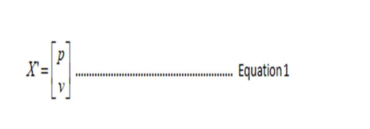
Let’s define the next predicted state of the coffee-carrying robot as a 2x1 matrix X of position and velocity. P and v are what are going to be estimated by the filter, so this is what you will pass into the filter. This is a very simple example. Your actual state matrix would be far more complex.
Let’s define the next predicted state of the coffee-carrying robot as a 2x1 matrix X of position and velocity. P and v are what are going to be estimated by the filter, so this is what you will pass into the filter. This is a very simple example. Your actual state matrix would be far more complex.
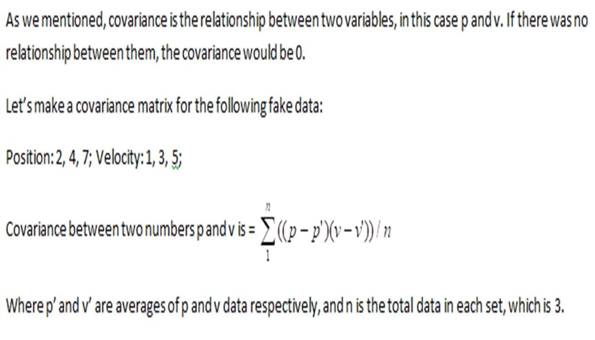
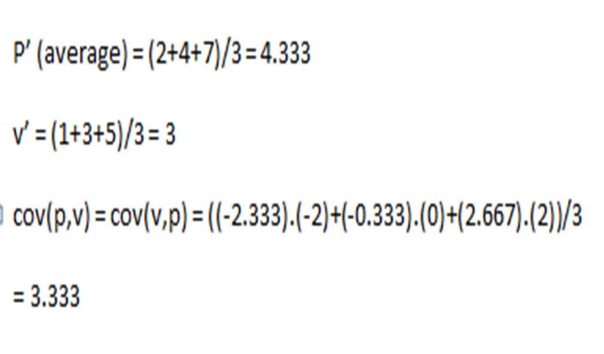
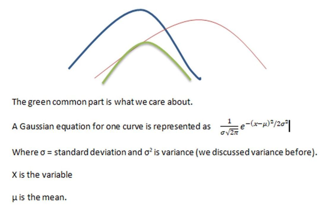
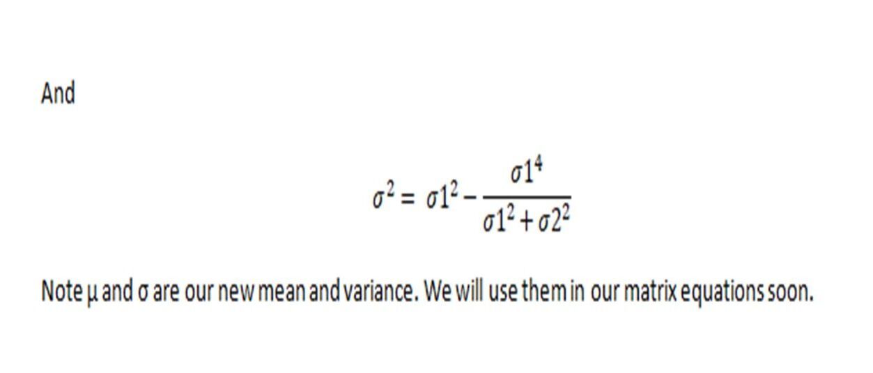
Sensor readings are Gaussian and there can be some covariance between them. Gaussian means they are distributed in a bell-curve fashion. In a bell curve, the mean (average) of all the data is in the center (vertical line in the below graph) and the data points are scattered around the mean to form a bell shape. The distance between each data point and the center (mean) is the variance (we also call it error), which would define how far each point is from the center (mean). Variance is usually squared in order to avoid a negative value and keep things simple:
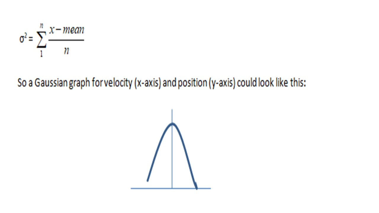
The data (some function of velocity / position) is scattered within and on the boundary of the curve. Most readings are around the mean.
Covariance means there is some type of relation between the inputs. In this case, we will assume there is some kind of relation between position and velocity. E.g. if the velocity of the robot is a big number, likely the position of the robot is further ahead.
The predicted state covariance (some relation) between the two variables velocity and position can be defined via a 2x2 covariance matrix, P.
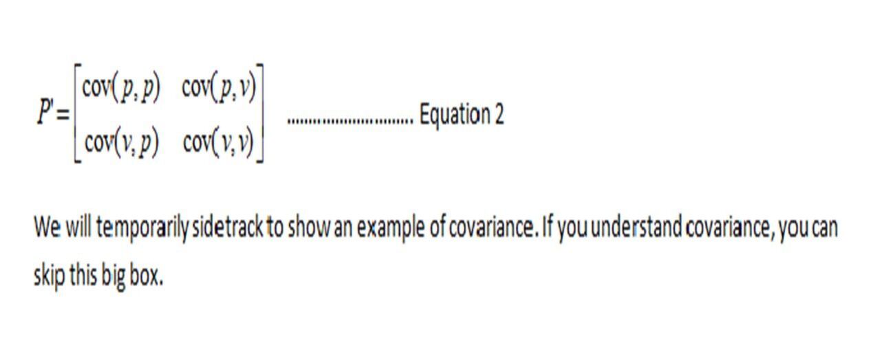

Now we have an idea for what a covariance matrix looks like and we also have predicted values for X’ and P’, where X’ is the state matrix of p and v, and P’ is the covariance state matrix of p and v. Together, P’ and X’ tell us about the next predicted state. Don’t confuse P and p. P is a covariance matrix while p is the position of our robot.
Now, we want to expand a bit more on the X’ matrix so we know how to calculate the position and velocity. Remember equation 1:
Now, we want to expand a bit more on the X’ matrix so we know how to calculate the position and velocity. Remember equation 1:

How do we arrive at p and v? There are some basic equations in physics called kinematic formulae. One of them is speed = distance /time or we will say velocity = distance/ time. We will assume there is no acceleration.
We will use a superscript to define the prediction and no superscript for time t-1. Don’t get too confused with the current / previous states. They will become clear as we move forward with an example, toward the end.
v’= distance / time
v’ = (p’ –p) / ∆t (this is just difference in position which is distance divided by difference in time between two positions)
Solving for predicted position p’ based on previous position p, previous velocity v and change in time:
p’ = p + v∆t ------- Equation A
Another kinematic equation from physics is the one involving velocity:
v’ = v +at (velocity = previous velocity + acceleration x time)
Because we are assuming acceleration = a = 0, we get:
v’ =v ----- Equation B
Sidetrack: From linear algebra, we know equations in the form
5x + 6y = C and
3x + 4y = D
can be represented as a matrix equation in the form:
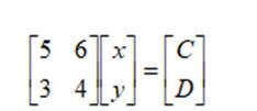
The [5 6 3 4] is the matrix of coefficients, [x y] the matrix of unknowns, and [c d] the matrix of constants. If you multiply the above matrices on the left of the equal sign, you will get the equations mentioned above.
Now, we can similarly write equations A and B in matrix form to give us the state matrix X:
Now, we can similarly write equations A and B in matrix form to give us the state matrix X:
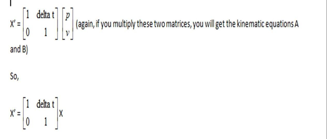
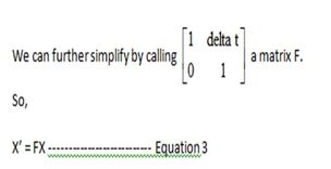
F is also called a state transition matrix or the matrix of coefficients. The state transition matrix shows how a state vector (X) will change over a time increment delta t. Remember this for the next section. X is the last state at time t-1, represented by a p v matrix.
But! But! But!
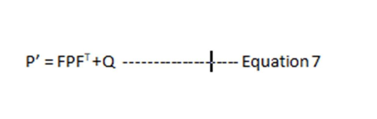
Remember, covariance exists between the variables p and v in X (we saw that in equation 2). So we need to convert Equation 3 into its covariant form somehow.
As luck would have it, there is some matrix rule that says:
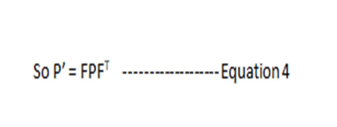
If cov(X) = P (Remember equation 2 where we said P is the covariance matrix of X?)
Then cov(FX) = FPFT (The superscript T (excuse formatting), is just the transpose of matrix F, implying rows become columns. You can google transpose of a matrix if you are very keen.)
Apply this to Equation 3.
But! But! But!
Remember, covariance exists between the variables p and v in X (we saw that in equation 2). So we need to convert Equation 3 into its covariant form somehow.
As luck would have it, there is some matrix rule that says:
If cov(X) = P (Remember equation 2 where we said P is the covariance matrix of X?)
Then cov(FX) = FPFT (The superscript T (excuse formatting), is just the transpose of matrix F, implying rows become columns. You can google transpose of a matrix if you are very keen.)
Apply this to Equation 3.
We Forgot About External Influences!
So far we have assumed the coffee-robot will meander about easily and bring the coffee right to me without much concern. In a “real” house, there may be broken tiles on the floors, stinky socks thrown about, castles erected from very expensive toy blocks etc. Basically, a bunch of evil forces preventing the coffee from coming to me! The robot’s navigation system may have to tell it to skirt the socks and the castle and the tiles, or stop and make a turn, or accelerate. So there are some external influences involved. If we understand these influences, we can add them to the original equation 3 for X’, provided we know what these external influences are.
Let’s assume we are adding acceleration as an external influence. There is another kinematic equation in physics that involves acceleration:
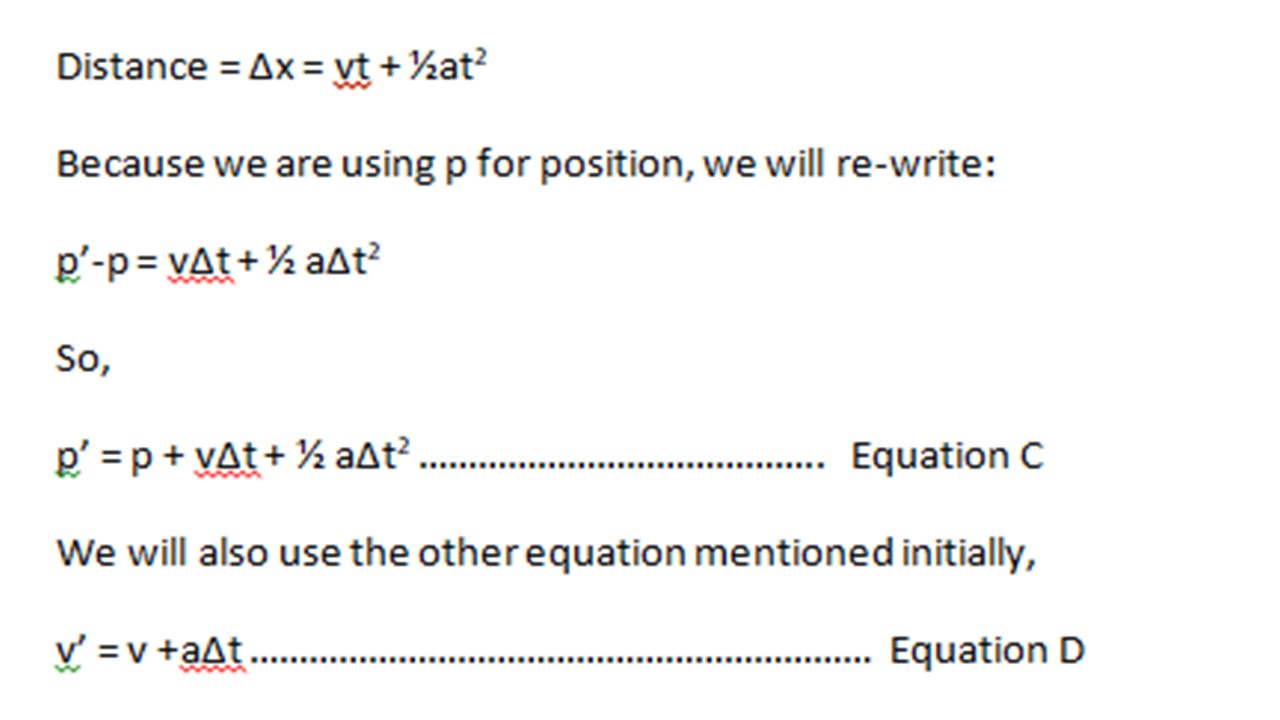
We can re-write the above as a matrix as we did before. The only difference is, we now have acceleration, which we are considering an external influence for the sake of understanding this further. Note, we did not define acceleration as part of the state matrix. Hence, it can be added as an input.
Remember from Equation 3 that X’ = FX
Now, from Equation C and D,
Remember from Equation 3 that X’ = FX
Now, from Equation C and D,
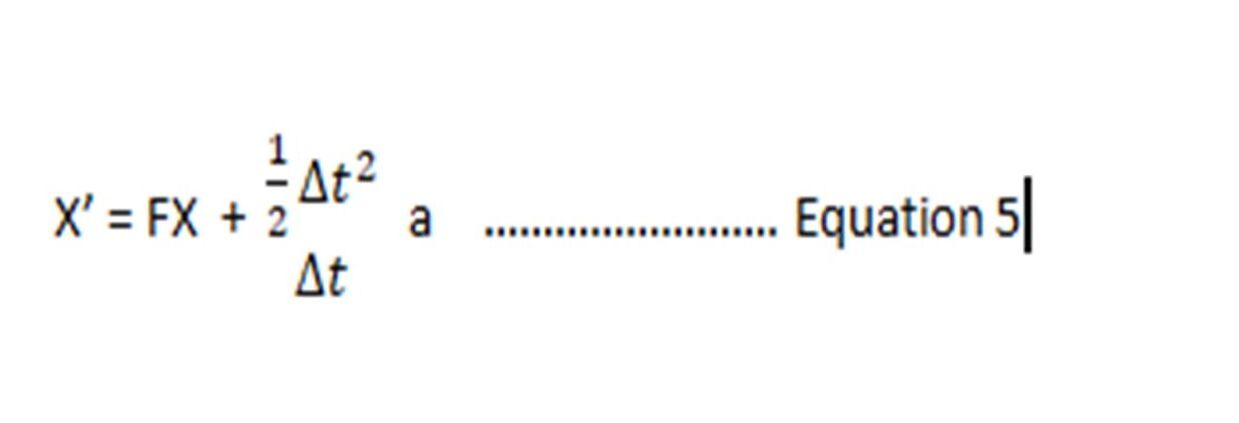
(note, due to the editor’s limitation, I have left out square brackets for the ∆t matrix)
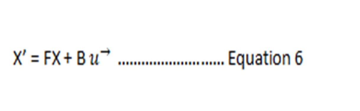
Remember I asked you to remember we can define a matrix of coefficients? We can do that again with Equation 5, where we can replace the delta matrix with some matrix B and the acceleration can be called some control vector, u ->
Remember I asked you to remember we can define a matrix of coefficients? We can do that again with Equation 5, where we can replace the delta matrix with some matrix B and the acceleration can be called some control vector, u ->
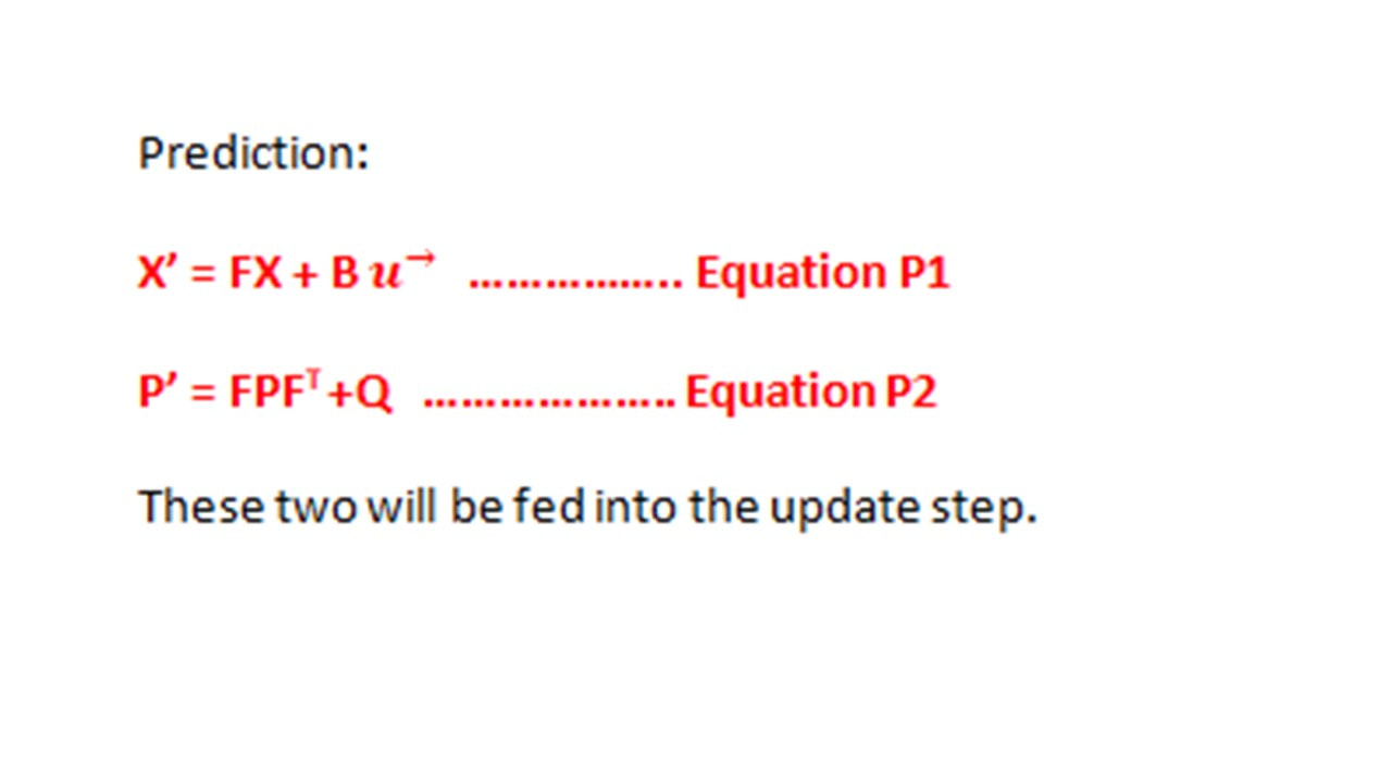
In the real world, there will be influences that are unseen. For example, a kid could suddenly come and stand in front of the robot. We did not know this would happen. Or the robot may have to stop, slow down, change direction because of a milk spill on the floor. These unknown external influences or random disturbances can be further added onto Equation 4 as a matrix for process covariance (noise /error). So we are adding more covariance (noise) to the original noise, or we are adding unknown noise to known noise.
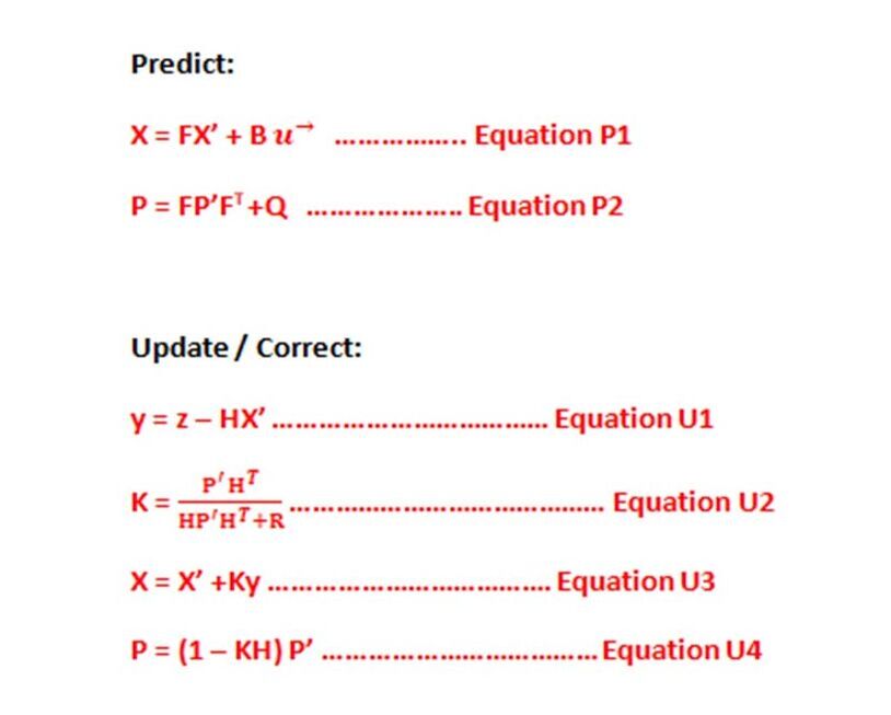
The Prediction Equations:
We have arrived at the Prediction step equations!
We have arrived at the Prediction step equations!
En route to the Update Equations – Keep Breathing Through It!
Now let’s try to make sense of the update step.
We had mentioned the sensors earlier. For any given measurement, there will be noise involved. In this step, we will add correction with respect to the noise, to the prediction we had in the prediction step, and produce a new set of X and P that we will feed back into the prediction step. Kapiche?
The actual measured sensor value, z will be the estimate state matrix X’ multiplied by some gain matrix or state transition matrix H, with noise added, y.
(y is just added because of uncertainty of equation … i.e. how much can we trust the equation? Or it can be added for random sensor noise)
H is playing the same role as F in Equation 3 or Equation P1. H can be used for scaling X’ so it can be subtracted from z (actual sensor measurement) as shown below.
Sometimes it’s possible z will have more measurements than our state matrix X’, because our state matrix may not require so many state variables. So H matrix plays a role in transforming X’ so it can be subtracted from z.
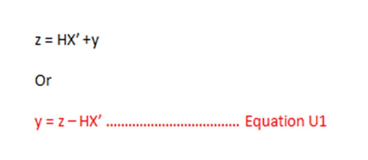
Here, we are just saying we will measure the difference between the measured sensor value and our estimate. Y is also called the residual and is the discrepancy between predicted and actual.
Our covariance for the sensor will be HPHT, the same way we had gotten to Equation 4, except we are using H instead of F.
Our covariance for the sensor will be HPHT, the same way we had gotten to Equation 4, except we are using H instead of F.
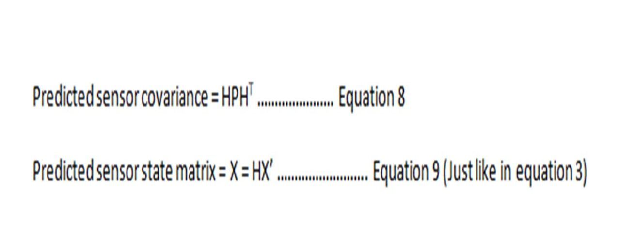
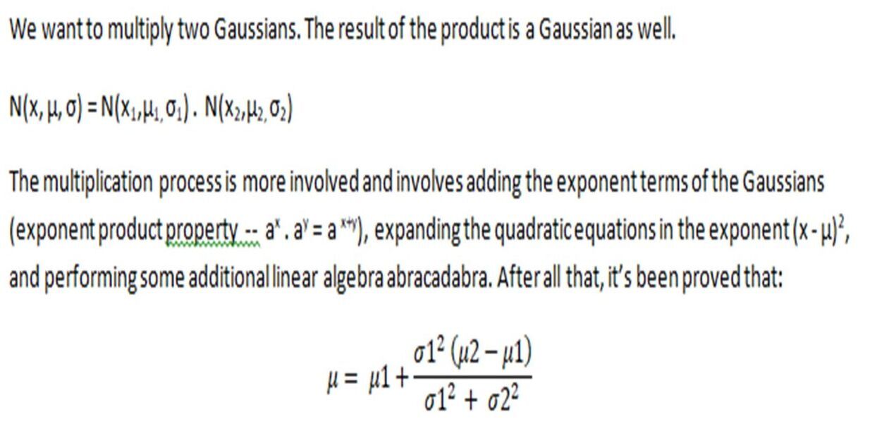
Now we have two Gaussians, one for our original predicted estimate HX’ and its covariance HPHT , and one for the measured sensor estimate, z, and its own covariance, R. These are both different. What is the probability of both being right? It is the product of individual probabilities of each reading. Each reading is a Gaussian probability distribution, as we mentioned before. So now we have two Gaussians. These need to be multiplied.
Let’s get back to our matrices.
From equations 8 and 9, remember our predicted sensor covariance = HPHT
Predicted state matrix for sensor = X = HX’
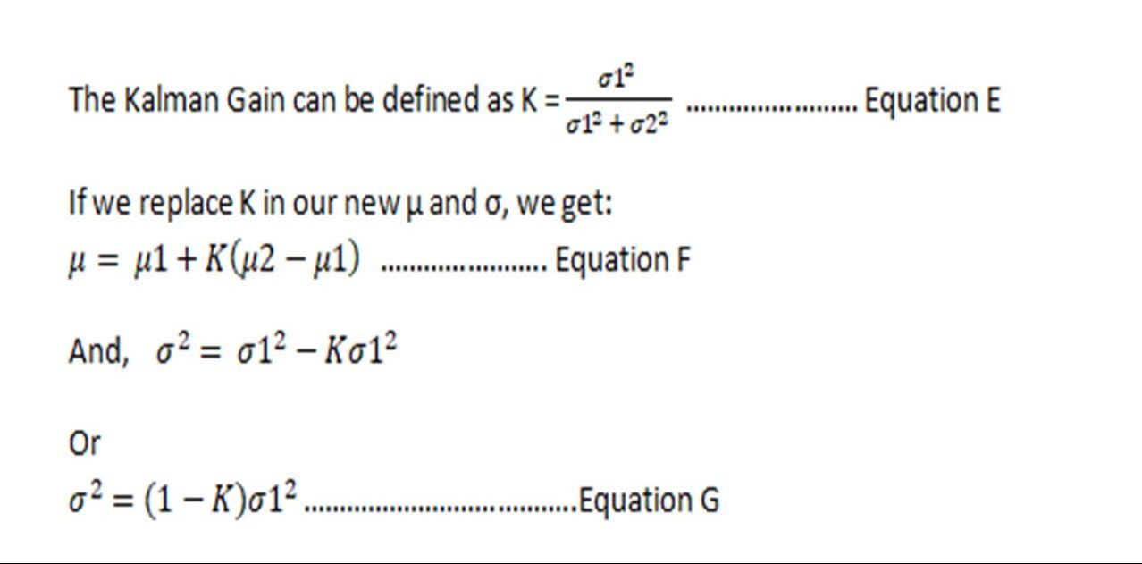
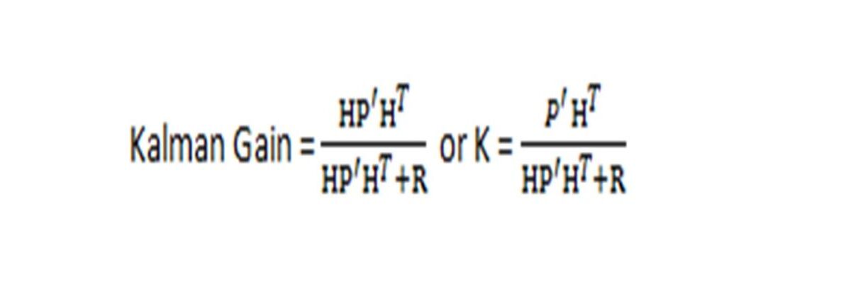
We also said R is the pre-defined variance of the sensor set by the factory, and z is the actual measured value from the sensor. We can implant the sensor covariance in equation E to get Kalman Gain:
From equations 8 and 9, remember our predicted sensor covariance = HPHT
Predicted state matrix for sensor = X = HX’
We also said R is the pre-defined variance of the sensor set by the factory, and z is the actual measured value from the sensor. We can implant the sensor covariance in equation E to get Kalman Gain:
Equation F becomes: new estimate = X= X’ +K (z – HX’)
And Equation G becomes: new covariance = P = (1-K) HP’HT or with some algebra work, P = (I – KH) P’
Where I is the identity matrix (a matrix A multiplied by I is A)
Out Update equations are:
And Equation G becomes: new covariance = P = (1-K) HP’HT or with some algebra work, P = (I – KH) P’
Where I is the identity matrix (a matrix A multiplied by I is A)
Out Update equations are:
Final Equations
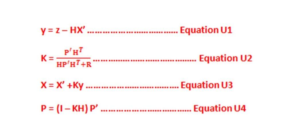
And we finally arrive at all our equations:
And we finally arrive at all our equations:
So, in the update step, we will take the difference between the measured sensor value and the predicted state, and the Kalman gain will decide whether to go with the ~ estimate or ~ measured sensor value.
If R (sensor error) is very high, then we can assume K is close to 0, and our X will be close to X’. And vice versa, if R is negligible, we will consider the difference between the measured sensor value and our estimate.
So in Equation U3, our new estimate is the previous estimate plus some weight of the difference between prediction and actual measured. X and Y will be fed back into the Predict step equations.
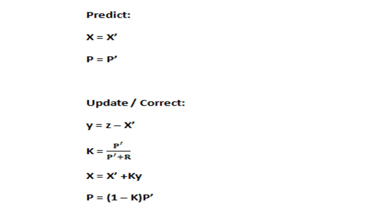
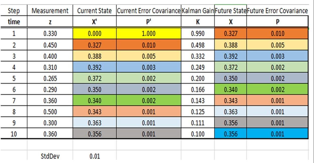
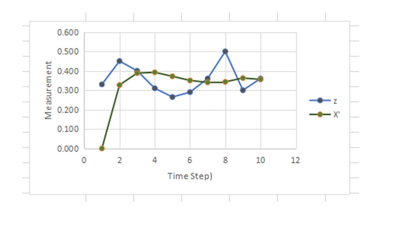
Example
The below example is simplified to show how calculations work. We will assume there is no F matrix, no H matrix, and no external noise. R = standard deviation of sensor = 0.01, and z is the measured sensor value in some units. We will assume it is just one value, so no matrix is required.
Also, to start with, X’ =0 and P’ = 1, because we have to start somewhere.
So our equations become:
References
Keywords: Basic Kalman Filter; Easy Kalman Filter; Kalman Filter for Dummies; Simple Kalman Filter
- https://www.intechopen.com/books/real-time-systems/kalman-filtering-and-its-real-time-applications
- https://www.cs.cornell.edu/courses/cs4758/2012sp/materials/MI63slides.pdf
- https://www.bzarg.com/p/how-a-kalman-filter-works-in-pictures/
- http://www.swarthmore.edu/NatSci/echeeve1/Ref/Kalman/ScalarKalman.html
- https://towardsdatascience.com/kalman-filter-interview-bdc39f3e6cf3
Keywords: Basic Kalman Filter; Easy Kalman Filter; Kalman Filter for Dummies; Simple Kalman Filter
P.S. Consider buying my picture book:
Softcover
Hardcover
Purchase via publisher
You can also visit Barnes&Noble or Chapters and order online.
Softcover
Hardcover
Purchase via publisher
You can also visit Barnes&Noble or Chapters and order online.
 RSS Feed
